Molecular geometry optimization
Description
Three types of the geometry can be optimized: the most stable (minimum energy) geometry, conical intersections between the electronic states, and the transition state (TS) geometry (or the saddle point on the potential energy surface).
In the optimizations, rather than using the exact Hessian, one can start using the approximate Hessian and update it according to the step taken. In the transition state search, the exact Hessian usually improves the convergence. The advanced quasi-newton optimization methods, eigenvector following (EF) algorithm and rational functional optimization (RFO) are implemented. In the minimum energy conical intersection (MECI) optimization, the molecular gradient is replaced by the sum of the energy difference gradient and the upper state gradient after projecting the degeneracy lifting vectors out (gradient projection). The minimum distance conical intersection (MDCI) can be also optimized by replacing the upper state gradient in MECI optimization with the distance vector to the reference geometry. In addition, the minimum energy path to the reactants and products from the saddle point can be calculated using the second order algorithm, without mass weighting.
The optimizer in BAGEL has been interfaced with an external molecular mechanics program, TINKER,
using which mixed quantum mechanics/molecular mechanics (QM/MM) optimization can be performed.
To perform this, the TINKER input files (keyword file tinkin.key and initial coordinate file tinkin.xyz)
should be provided in tinker1 and tinker2 subdirectories, respectively.
The testgrad program in the TINKER package should be installed in $PATH.
Note that the use of the internal coordinate is not supported in the QM/MM case, or more generally when there are external charges.
The output contains the gradient evaluation progress at the first step of the optimization, and the status of the optimization.
The other information, including the quantum chemistry calculations at the optimization steps, are deposited in the file opt.log.
The history of the optimization and the final geometry are also saved in the MOLDEN files opt_history.molden and opt.molden,
and can be read by MOLDEN.
Keywords
Required Keywords
title
optimize: Optimize geometry.opttype
energy: find the most stable geometry.conical or meci: find the minimum energy conical intersections, according to gradient projection method.mdci: find the minimum distance conical intersections, according to modified gradient projection method.transition: find the transition state geometry (saddle point on the PES).mep: find the minimum energy path using the second-order algorithm, starting from the transition state geometry.target
0: the ground state.1: the first excited state, and so on.target2
0: the ground state.1: the first excited state, and so on.method
Convergence Criteria
maxgrad
maxdisp
maxchange
Optional Keywords (Universal)
algorithm
ef: Eigenvector-following (EF) algorithm.rfo: Rational functional optimization algorithm.nr: Newton–Raphson algorithm.maxstep
internal
true: use internal coordinates.false: use Cartesian coordinates.redundant
true: use redundant internal coordinate.false: use delocalized internal coordinate.maxiter
maxziter
explicitbond
true: add explicit bonds. (“explicit” block required, see below for example)false: do not add explicit bonds.explicit
numerical
true: use numerical gradient.false: use analytical gradient.numerical_dx
hess_update
flowchart: use flowchart update. This automatically decides according to the shape of PES.bfgs: use BFGS scheme.psb: use PSB scheme.sr1: use SR1 scheme.bofill: use the Bofill’s scheme for combining PSB and SR1.noupdate: does not update Hessian at all.hess_approx
true: use approximate Hessian.false: calculate numerical Hessian first, and start the optimization using the Hessian.adaptive
true: use adaptive maximum stepsize.false: use fixed maximum stepsize.molden
Optional Keywords (Conical Intersection Optimization)
nacmtype
full: use full nonadiabatic coupling.interstate: use interstate coupling.etf: use nonadiabatic coupling with built-in electronic translational factor (ETF).noweight: use interstate coupling without weighting it by energy gap.thielc3
thielc4
mdci_reference_geometry
true: specify reference geometry in the refgeom block.false: the first geometry for optimization is considered as the reference geometry.refgeom
molecule block.Optional Keywords (Minimum Energy Path)
mep_direction
1: use the direction of the lowest eigenvector.0: use gradient.-1: use the opposite direction of the lowest eigenvector.Optional Keywords (QM/MM)
qmmm
true: do QM/MM optimization.false: do gas phase optimization.qmmm_program
tinker: do QM/MM optimization with TINKER.Example
This optimizes the ground state geometry of benzophenone.
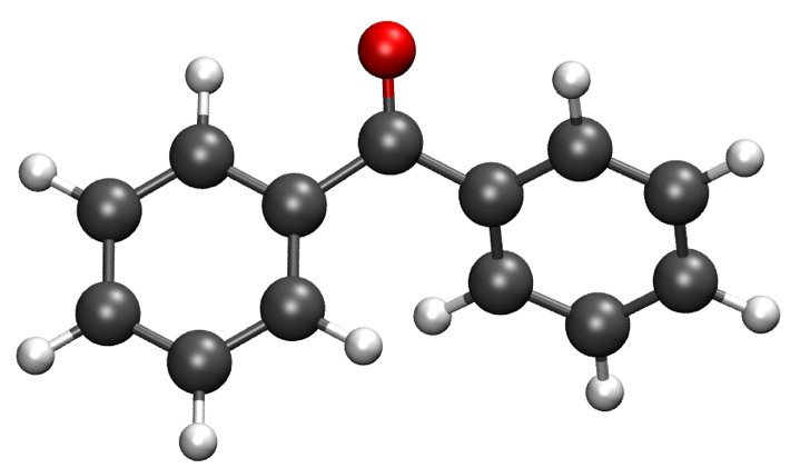
The benzophenone molecule with carbon atoms in grey, oxygen in red, and hydrogen in white.
Sample input
 { "bagel" : [

 {
   "title" : "molecule",
   "basis" : "cc-pvdz",
   "df_basis" : "cc-pvdz-jkfit",
   "angstrom" : false,
   "geometry" : [
   { "atom" : "C", "xyz" : [     -2.002493,     -2.027773,      0.004882 ] },
   { "atom" : "C", "xyz" : [     -2.506057,     -4.613700,      0.009896 ] },
   { "atom" : "C", "xyz" : [      0.536515,     -1.276360,      0.003515 ] },
   { "atom" : "C", "xyz" : [     -0.558724,     -6.375134,      0.013503 ] },
   { "atom" : "H", "xyz" : [     -4.396140,     -5.341490,      0.011057 ] },
   { "atom" : "C", "xyz" : [      2.478233,     -3.024614,      0.007049 ] },
   { "atom" : "H", "xyz" : [      0.959539,      0.714937,     -0.000292 ] },
   { "atom" : "C", "xyz" : [      1.936441,     -5.592475,      0.012127 ] },
   { "atom" : "H", "xyz" : [     -1.012481,     -8.367883,      0.017419 ] },
   { "atom" : "H", "xyz" : [      4.418042,     -2.380738,      0.005919 ] },
   { "atom" : "H", "xyz" : [      3.448750,     -6.968581,      0.014980 ] },
   { "atom" : "C", "xyz" : [     -6.758666,     -0.057378,      0.001157 ] },
   { "atom" : "C", "xyz" : [     -8.231109,     -2.241648,      0.000224 ] },
   { "atom" : "C", "xyz" : [     -8.022986,      2.269249,      0.001194 ] },
   { "atom" : "C", "xyz" : [    -10.853532,     -2.110536,     -0.000769 ] },
   { "atom" : "H", "xyz" : [     -7.410047,     -4.093049,      0.000224 ] },
   { "atom" : "C", "xyz" : [    -10.632155,      2.405932,      0.000369 ] },
   { "atom" : "H", "xyz" : [     -6.913797,      3.976253,      0.001805 ] },
   { "atom" : "C", "xyz" : [    -12.064741,      0.207004,     -0.000695 ] },
   { "atom" : "H", "xyz" : [    -11.941318,     -3.840822,     -0.001614 ] },
   { "atom" : "H", "xyz" : [    -11.548963,      4.232744,      0.000447 ] },
   { "atom" : "H", "xyz" : [    -14.107194,      0.302907,     -0.001460 ] },
   { "atom" : "C", "xyz" : [     -3.892311,      0.136360,      0.001267 ] },
   { "atom" : "O", "xyz" : [     -3.026383,      2.227189,     -0.001563 ] }
   ]
 },

 {
   "title" : "optimize",
    "method" : [ {
     "title" : "hf",
     "thresh" : 1.0e-12
   } ]
 }
]}
Using the same molecule block, a geometry optimization with XMS-CASPT2 can be performed. In this particular example as is often the case, the active keyword is used to select the orbitals for the active space that includes 4 electrons and 3 orbitals. Three sets of \(\pi\) and \(\pi^*\) orbitals localized on the phenyl rings are included along with one non-bonding orbital (oxygen lone pair). The casscf orbitals are state-averaged over three states. Since a multistate calculation is performed, the user must specify which state is to be optimized (the target). In this example, we optimize the ground state.
{
  "title" : "casscf",
  "nstate" : 2,
  "nclosed" : 46,
  "nact" : 3,
  "active" : [37, 44, 49]
},

{
  "title" : "optimize",
   "target" : 0,
   "method" : [ {
     "title" : "caspt2",
       "smith" : {
         "method" : "caspt2",
         "ms" : "true",
         "xms" : "true",
         "sssr" : "true",
         "shift" : 0.2,
         "frozen" : true
     },
     "nstate" : 2,
     "nact" : 3,
     "nclosed" : 46
   } ]
 }

 ]}
Example: Explicit bond
This optimizes the ground state geometry of a benzene dimer using MP2. The internal coordinates complemented by two explicit bonds between the carbon atoms in the monomers are used.
{ "bagel" : [

{
  "title" : "molecule",
  "basis" : "sto-3g",
  "df_basis" : "svp",
  "angstrom" : false,
  "geometry" : [
    {"atom" :"C", "xyz" : [    0.00000000000000,     0.00000000000000,     2.64112304663605] },
    {"atom" :"C", "xyz" : [    2.28770766388446,     0.00000000000000,     1.32067631141874] },
    {"atom" :"C", "xyz" : [    2.28770047235649,     0.00000000000000,    -1.32071294538560] },
    {"atom" :"C", "xyz" : [    0.00000000000000,     0.00000000000000,    -2.64114665444819] },
    {"atom" :"C", "xyz" : [   -2.28770047235649,     0.00000000000000,    -1.32071294538560] },
    {"atom" :"C", "xyz" : [   -2.28770766388446,     0.00000000000000,     1.32067631141874] },
    {"atom" :"H", "xyz" : [    4.07221260176630,     0.00000000000000,     2.35164689765998] },
    {"atom" :"H", "xyz" : [    4.07221517814719,     0.00000000000000,    -2.35163163881380] },
    {"atom" :"H", "xyz" : [    0.00000000000000,     0.00000000000000,    -4.70191324441092] },
    {"atom" :"H", "xyz" : [   -4.07221517814719,     0.00000000000000,    -2.35163163881380] },
    {"atom" :"H", "xyz" : [   -4.07221260176630,     0.00000000000000,     2.35164689765998] },
    {"atom" :"H", "xyz" : [    0.00000000000000,     0.00000000000000,     4.70197960246451] },
    {"atom" :"C", "xyz" : [    0.00000000000000,     4.00000000000000,     2.64112304663605] },
    {"atom" :"C", "xyz" : [    2.28770766388446,     4.00000000000000,     1.32067631141874] },
    {"atom" :"C", "xyz" : [    2.28770047235649,     4.00000000000000,    -1.32071294538560] },
    {"atom" :"C", "xyz" : [    0.00000000000000,     4.00000000000000,    -2.64114665444819] },
    {"atom" :"C", "xyz" : [   -2.28770047235649,     4.00000000000000,    -1.32071294538560] },
    {"atom" :"C", "xyz" : [   -2.28770766388446,     4.00000000000000,     1.32067631141874] },
    {"atom" :"H", "xyz" : [    4.07221260176630,     4.00000000000000,     2.35164689765998] },
    {"atom" :"H", "xyz" : [    4.07221517814719,     4.00000000000000,    -2.35163163881380] },
    {"atom" :"H", "xyz" : [    0.00000000000000,     4.00000000000000,    -4.70191324441092] },
    {"atom" :"H", "xyz" : [   -4.07221517814719,     4.00000000000000,    -2.35163163881380] },
    {"atom" :"H", "xyz" : [   -4.07221260176630,     4.00000000000000,     2.35164689765998] },
    {"atom" :"H", "xyz" : [    0.00000000000000,     4.00000000000000,     4.70197960246451] }
  ]
},

{
  "title" : "optimize",
  "target" : 0,
  "explicitbond" : true,
  "explicit" : [
    { "pair" : [1, 13]},
    { "pair" : [4, 17]}
],
"method" : [ {
  "title" : "mp2"
} ]
}

]}
References
Description of Reference |
Reference |
|---|---|
Eigenvector following algorithm |
J. Baker, J. Comput. Chem. 7, 385 (1986). |
Rational functional optimization algorithm |
A. Banerjee, N. Adams, J. Simons, and R. J. Shepard, J. Phys. Chem. 89, 52 (1985). |
Second-order minimum energy path search |
C. Gonzalez and H. B. Schlegel, J. Chem. Phys. 90, 2154 (1989). |
Gradient projection algorithm |
M. J. Bearpark, M. A. Robb, and H. B. Schlegel, Chem. Phys. Lett. 223, 269 (1994). |
Flowchart method |
A. B. Birkholz and H. B. Schlegel, Theor. Chem. Acc. 135, 84 (2016). |
The Bofill’s update for TS optimization |
J. M. Bofill, J. Comput. Chem. 15, 1 (1994). |
ETF in nonadiabatic coupling |
S. Fatehi and J. E. Subotnik, J. Phys. Chem. Lett. 3, 2039 (2012). |
Thiel’s conical intersection parameters |
T. W. Keal, A. Koslowski, and W. Thiel, Theor. Chem. Acc. 118, 837 (2007). |